SigFit allows the user to compute the rigid-body motions, changes in radius-of-curvature, and surface RMS errors of optical surfaces due to three types of dynamic loads: transient, harmonic, and random.
While transient and harmonic response results from a finite element analysis may be processed as part of the standard polynomial fitting routine, the advanced dynamics capabilities in most codes are often optional features. Furthermore, quantities such as surface RMS error and change in radius-of-curvature cannot be computed within the random response capabilities of the finite element codes supported by SigFit.
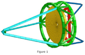 SigFit uses modal analysis techniques to decompose displacements from modal analyses into optically meaningful quantities before forced response analysis is performed. The only finite element results required are the modeshapes and corresponding natural frequencies. To illustrate these capabilities, results are shown below for the primary mirror of the telescope model shown in Figure 1.
Harmonic Response
Harmonic responses of optical surfaces due to tonal inputs may be computed with modal harmonic analysis. Loading definition consists of a spatial dependence specified as a nodal load vector and a frequency dependence specified as tabular data. Damping may be specified as constant modal damping, frequency dependent modal damping, a structural damping constant, or damping matrices exported from MSC Nastran with a Sigmadyne supplied DMAP alter. The frequency range, frequency step size, and number of extra frequencies to be evaluated near the natural frequencies are entered by the user. The user may also manually enter a frequency dependent variation to the harmonic loads in either linear-linear or log-log format.
The output of the harmonic analysis in the form of frequency response functions, as shown in the truncated output list in Table 1, is given in the ASCII output file as a list of optical surface rigid-body motions, change in radius-of-curvature, and surface RMS error at each forcing frequency.
Table 1
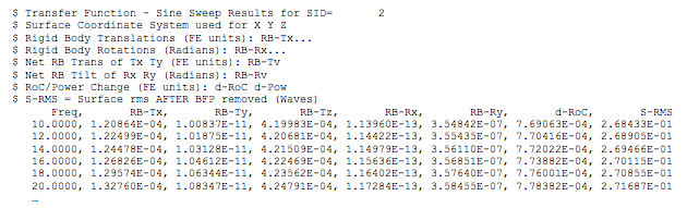
The file is written as a .csv file which is easily opened in Microsoft Excel where plots of the response functions can be made as shown in Figure 2.
Random Response
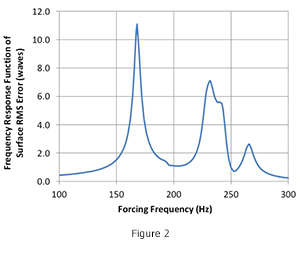
With an input power spectral density as shown in Figure 3 SigFit can compute the random forced response of optical surfaces. A harmonic analysis as described above is defined in combination with the input power spectral density of the loading. The power spectral density break points can be input manually or obtained from a file in either linear-linear or log-log form.
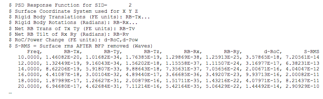
The output of the random analysis includes the response power spectral densities of optical surface rigid-body motions, change in radius-of-curvature, and surface RMS error given in the ASCII output file. A truncated example is listed in Table 2 and plotted in Microsoft Excel in Figure 4.
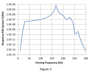
Table 2
As an aid to performing design trades, SigFit lists the percent contribution of each dynamic mode to the overall response power spectral density for each result type. This listing aids the user in understanding which modes require attention in order to improve the system’s performance. An example listing is shown in Table 3 with the corresponding contribution plot created in Microsoft Excel shown in Figure 5.
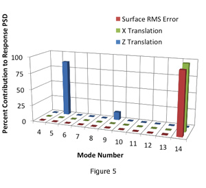
Table 3
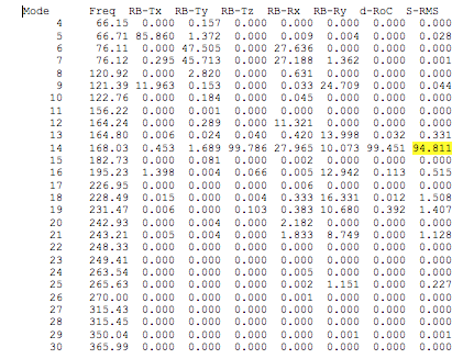
The data in Table 3 and the graphic in Figure 4 indicate that in order to reduce the surface RMS error, efforts should be concentrated on reducing the response of mode 14, and in order to reduce the X translation, efforts should be concentrated on reducing the response of mode 2 with some attention to mode 9.
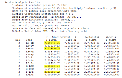
SigFit’s random response results output concludes with a random response summary giving the 1 sigma and 3 sigma limits on response for each response type. The response types consist of rigid body motions including vector sums, change in radius-of-curvature, and surface RMS error.
Table 4
Transient Response
Responses of optical surfaces due to time dependent loads are computed by SigFit using modal transient analysis. Loading definition consists of a spatial dependence specified as a nodal load vector and a time dependence specified as tabular data. SigFit can also automatically generate the time dependence for constant and sinusoidal loads. Damping may be specified as constant modal damping, frequency dependent modal damping, a structural damping constant, or damping matrices exported from MSC Nastran with a Sigmadyne supplied DMAP alter. The time step and duration used in the analysis is user controllable as well as the times at which results are printed. This allows the user complete control to choose enough time steps for the transient analysis calculations while limiting the results to only what is needed. Results are given in the ASCII output file as a list of optical surface rigid-body motions, change in radius-of-curvature, and surface RMS error at each time step for which output is requested.